Connecting to Google Cloud Storage in ArcGIS Pro

This posting is for a reader from Australia who asked about how to connect to a Google Cloud Storage in ArcGIS Pro. So, here it is.

In my previous post, I wrote about how to access cloud optimized geotiffs (COGs) stored on AWS - you should be able to connect to a Google Cloud Storage as detailed in those previous posts, EXCEPT if you are using ArcGIS Pro 2.9.2. This is the version I’m using and I don’t know if this is also true with versions 2.9 and 2.9.1 as well.

ArcGIS Pro 2.9.2 — Error with New Cloud Storage Connection Tool

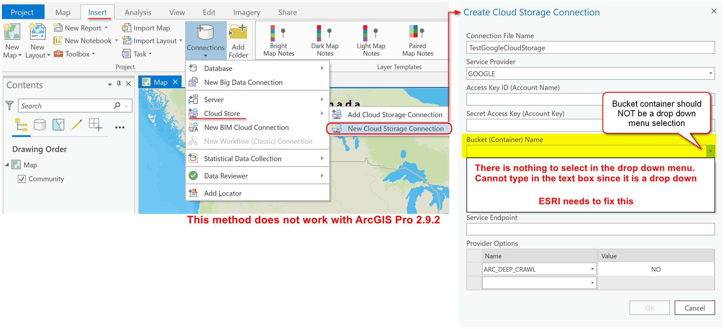
If you are using ArcGIS Pro 2.9.2 the Insert >> Connections >> Cloud Store >> New Cloud Storage Connection method will not work. The reason is because the text box where you input the Bucket container is a drop down menu selection - the Bucket Contain parameter should be an text box input not a drop down menu since there is nothing to select and you cannot type an input in the box. See the image for a visual explanation - this is something that ESRI should fix.

Create Cloud Storage Connection File

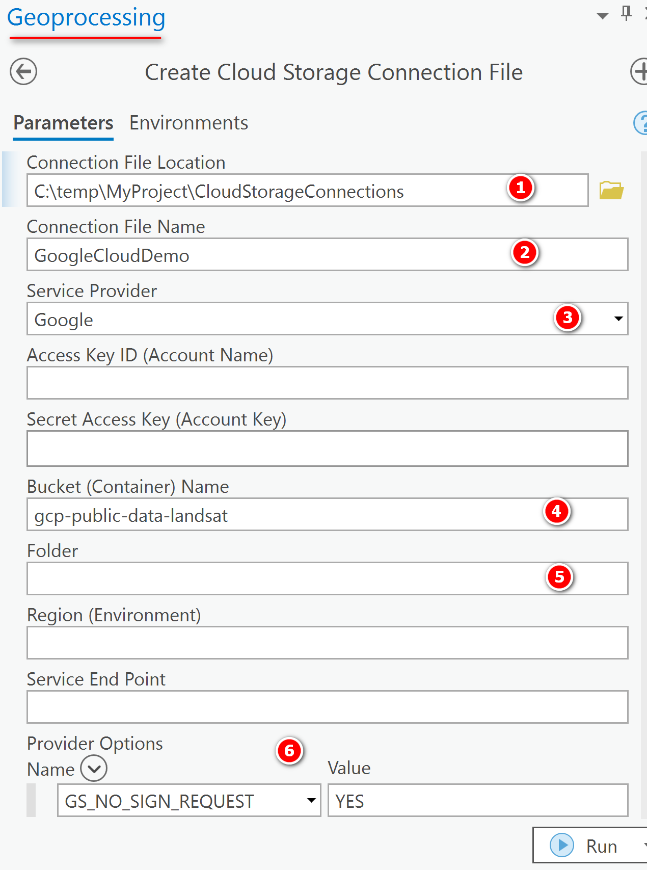
Since the method above doesn’t work, this is a work-around. Go to Analysis tab >> Tools to display the Geoprocessing pane. Then either search for the tool, Create Cloud Storage Connection File. This tool can also be found under Data Management Tools >> Workspace >> Create Cloud Storage Connection File.

In the Create Cloud Storage Connection File, enter your own parameters. Here is my example. I am connecting to a public Landsat imagery on Google Cloud (Bucket container is gcp-public-data-landsat). I left the Access Key ID and Secret Access Key blank since it’s a public source. Click the Run button after you fill in your options.

Add Cloud Storage Connection

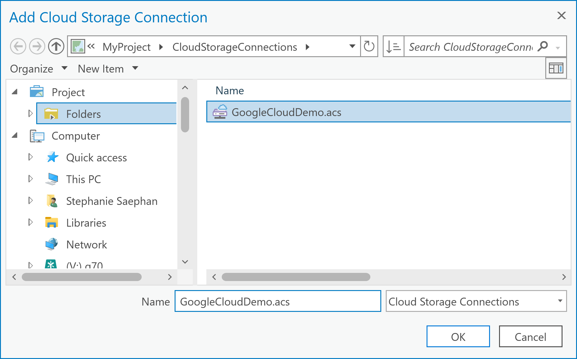
After the tool has successfully create a connection file then you can add the cloud storage connect just created. There are two ways you can do add an existing cloud storage connection:

1. Go Insert tab >> Connections >> Add Cloud Storage Connection

2. In Catalog pane >> Right click on empty space >> Add Cloud Storage Connection

In the dialog window, find where you stored the connection file and add it

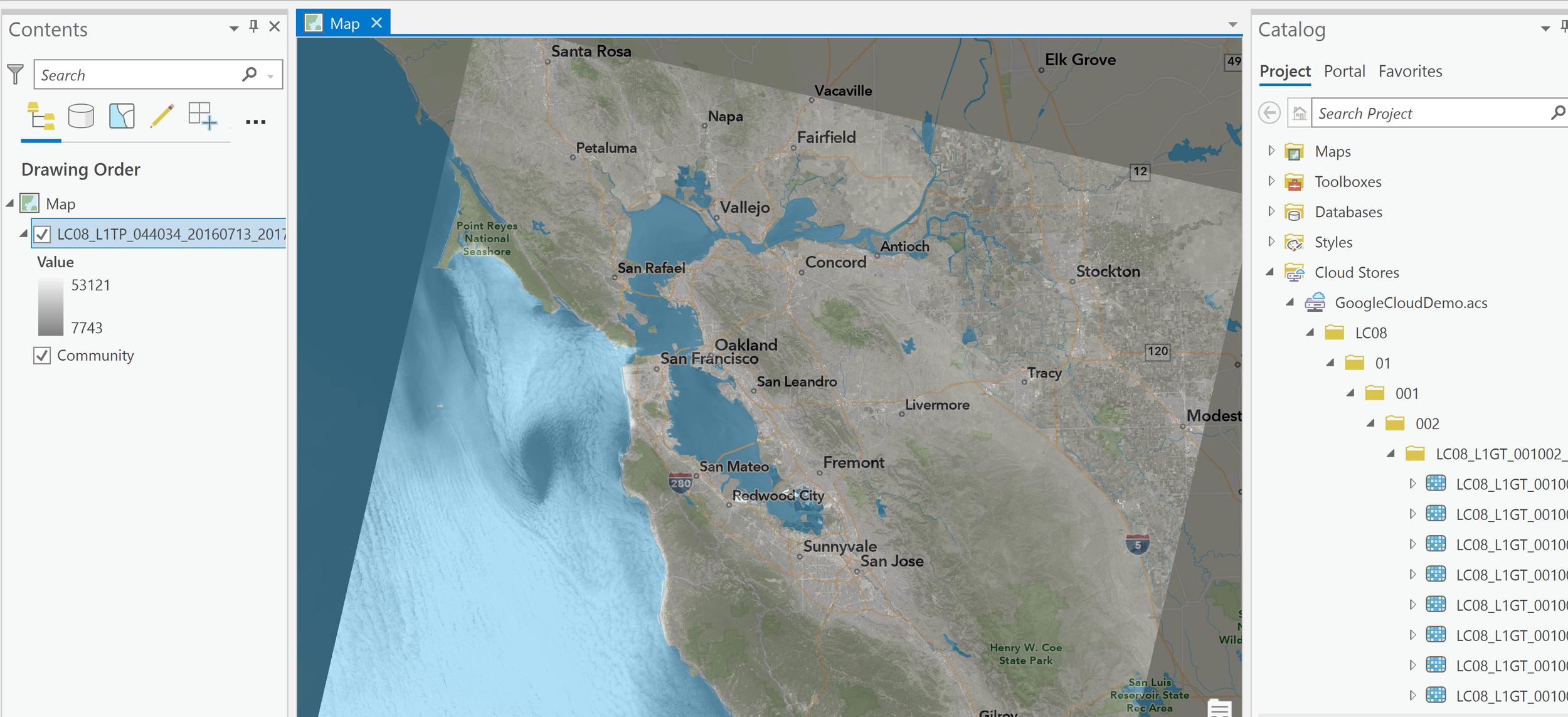
In the Catalog panel, navigate to your Cloud Stores connection and add in data to your map. See example below.

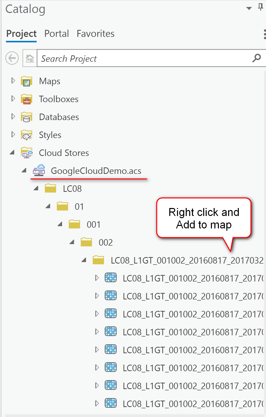
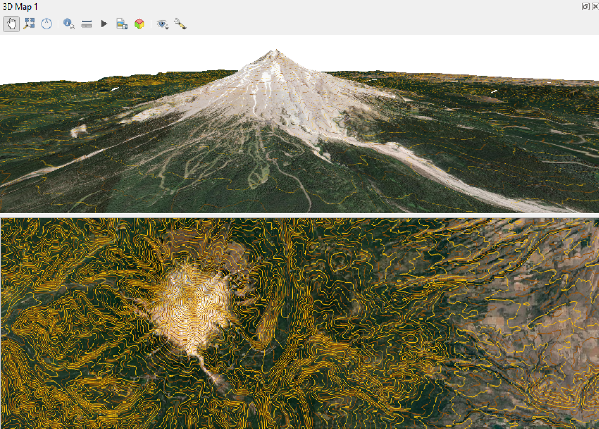
Here’s a look at one of the Landsat imagery from the public Google Cloud store above.

And that’s it for this post. Thanks for reading, and if you have a topic you would like me to write about let me know via email. I can’t promise anything - I like to know what my readers are interested in, and if I can help other then all the better for the GIS community.

Until next time :) Happy GIS-ing!

DEM and Contour Visualization in QGIS

This short write up is a follow up to the previous tutorial on creating contours from SRTM DEM. Here are some quick tips and tricks for visualizing contours and DEM in QGIS. I am using QGIS v3.22 so if you are using an older version of QGIS the visualization/rendering options may not be available. I am also using the SRTM DEM (e.g. N45W122.hgt) that I downloaded for Mount Hood area from the previous tutorial on creating contours from SRTM DEM.

Tip 1: Contour Rendering

Instead of using the Raster >> Extraction >> Contour tool to generate contours from a DEM, you can just apply the Contour rendering style on the DEM raster. Note though this is only for visualization purposes. Under Symbology, select Render Type = Contours. There are options to create contour intervals and index contours. See an example below with contours displayed at 10 meter intervals with index contours every 50 meters.

Contour rendering options for DEM

Tip 2 : Hillshade Rendering

You can also make a copy of the DEM (copy and paste raster in the TOC) and apply a hillshade rendering as well to get a 3D-ish visualization on the DEM. Play around with the different options to see what will give you the best result.

Hillshade rendering options. Note: Hillshading on my .hgt DEM came out really dark.

Here is an example of my contours rendering on top of a hillshade and a single pseudocolor option.

Left: Contour (index = darker line) on top of ESRI terrain imgaery; Right: Contour (index = darker lines) on top of SRTM DEM (N45W122.hgt) singleband pseudocolor

Tip 3: 3D Map View

Create a 3D map view along with a 2D view of the contours. Go to View menu >> New 3D Map View. You may get a warning popup that 3D Map View doesn’t support unprojected coordinate systems - in this case, just change your project’s coordinate system (e.g. WGS84 UTM Zone 10 meters) then open the 3D map view again.

In the 3D Map window, make sure you change the Terrain configuration to use the DEM raster (the default is a flat flat terrain view). See example below: Type = DEM (raster layer) and Elevation = DEM file (e.g. N45W122.hgt).

Here is an example, showing the contour rendering on top of Google aerial image in a 2D map view and a 3D map view

That’s all the tips I have for now. As always thanks for reading.