
I haven't done remote sensing work in a long while and have been wanting to get back into. Remote sensing is a great complement to GIS, and I've been looking for a case study to do a short tutorial. I thought the recent flooding on Kauai Island on April 14-15, 2018 would be a good case to do some flood mapping using remote sensing techniques.
Background:
The Island of Kauai is not called the Garden Isle for no reason - it is one of the rainiest place on Earth. On April 14-15, 2018 unprecedented rains caused major flooding and a series of landslides on Kauai. The National Weather Service recorded 27.52 inches (685 mm) of rainfall in the Hanalei area during the 24-hour period from April 14 to the 15. After the flooding, the County of Kauai was declared a state of emergency.
More info of the flooding event can be found here: http://floodlist.com/america/usa/record-rainfall-floods-hawaii0april-2018
Workflow/Requirements:
Here is the work flow plan and requirements for this tutorial:
Download Sentinel-1 data - require registration/sign up (free)
Download and install SNAP software (if you don't already have it)
Pre-processing - calibrate and speckle filtering of data
Determine flooded areas - threshold binning (binarization, unsupervised classification)
Post-processing - geometric correction of data (apply map projection)
View resulting flood areas in GIS (e.g. QGIS, Google Earth, or ArcGIS assuming you have a GIS software already)
Step 1: Download Sentinel-1 Imagery
Assessment of flooded areas can be done using radar data, such as the Sentinel-1 SAR imagery provided by the European Space Agency (ESA). For this example, I'm using Sentinel-1 Level-1 Ground Range Detected (GRD) data which already has some basic pre-processing done on it. More info about the Sentinel missions, products, and uses can be found on the Sentinel Online Website. Access to the Sentinel data is provided through the Copernicus Open Access Hub. Although the data is free to use, you will need to register or sign up first before you can download the data.
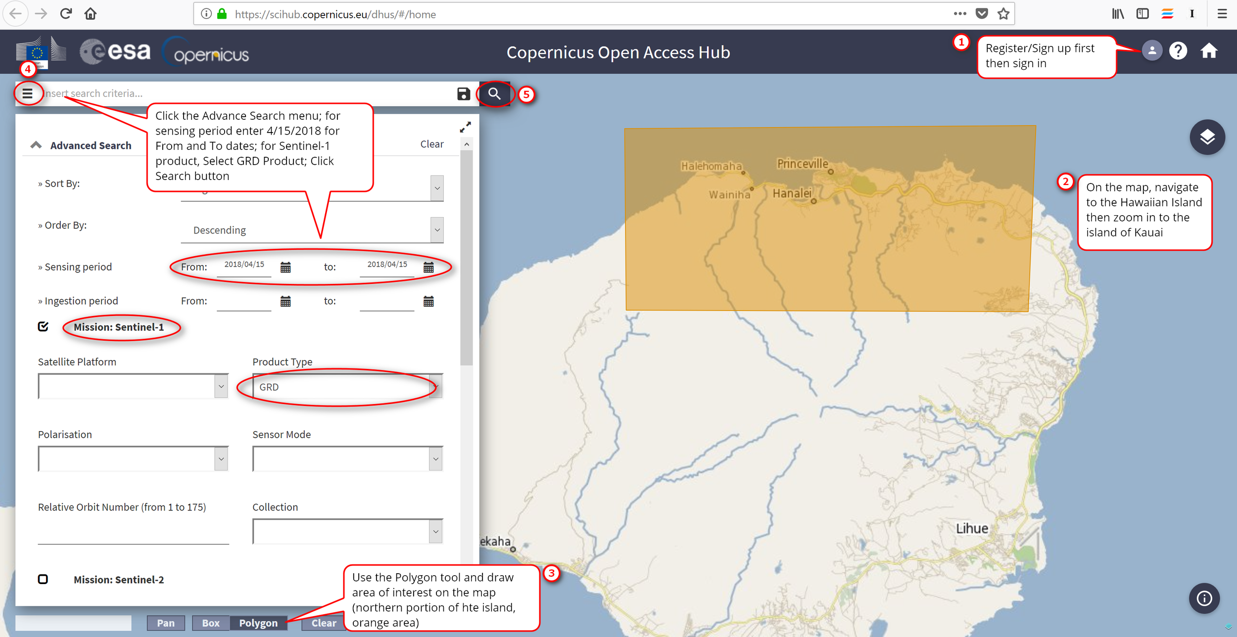
Go to Copernicus Open Access Hub:
Register or sign up for a free account then log in
On the map, navigate to the Hawaiian Islands and zoom in to the island of Kauai
Use the Polygon tool (in the bottom left, box tool doesn't seem to work) and draw an area of interest on Kauai (northern portion of the island)
Click the Advance Search menu (in top left) and use the following search parameters
Sensing Period: From = 4/15/2018, To = 4/15/2018
Mission Sentinel-1: Product Type = GRD
Note: there is only 1 image for Kauai taken on the date specified so there's no need to include other parameter criteria
Click the Search button when done
There should only be 1 result based on the search criteria for the area of interest. Note: when you click the link to download the file, you may be asked again to login (think this might be a time out issue on the Copernicus site).

Notice the available imagery is Level -1 Ground Range Detected (GRD) Sentinel-1 C-band (SAR-C) data collected in Interferometric Wide (IW) mode, allowing for an image acquisition over a 250km swath with resolution of 10m (5x20m).
Step 2: Download and Install SNAP
SNAP is a application developed by the ESA to work with Sentinel data. You will need to download and install the appropriate software for your computer. I am using the Windows 64bit version of the Sentinel Toolbox.
Download and install the appropriate version on the Sentinel Toolbox for your computer

Step 3: Explore the Image and Create Subset
After you've install the SNAP application, you can use it to open and explore the Sentinel-1 image you downloaded previously. The SNAP application can open the zipped file without need to unzip it first.
In the SNAP application >> Open Product >> S1A_IW_GRDH_1SDV_20180415.zip (file downloaded earlier) >> Open
The Product Explorer Panel on the left shows relevant information/metadata related to the Sentinel data. You can right click on any of the file/item to get a context menu to view properties related to that item.
Under Bands, you'll see that for each polarization (VV + VH or HH + HV), there are 2 bands (Amplitude and Intensity). Intensity band is a virtual band and is just a square of the amplitude. To view an image of a Band, double click it and an image will be created for viewing in the left panel. Double click on the Intensity_VV band to view it - this is the band being used.
Note: Although any of the polarization/band can be used to analyze flooding extent, some studies have shown that VV gives a slight advantage when delineate flooding when using Sentinel‐1 data. This article, "Multi‐temporal synthetic aperture radar flood mapping using change detection" provides a good comparison using different polarizations for delineating flooding using Sentinel data.

To create a subset a portion of the island, first zoom in to the extent of the area you want to subset - which in this case is the northern portion of the island where Hanelei town is located.

Create the subset, go to Raster Menu >> Subset
In the Specify Product Subset window, the lat/long coordinates for the area of interest should already be filled in based on the zoomed in map extent. Click OK to create subset

The newly created subset image should show up in the Product Explorer panel and look something like this.

Step 4: Pre-Processing - Calibration and Speckle Filtering
Pre-processing calibration and speckle filtering here is done on the subset image you created in step 3 above. The pixel values in a SAR imagery can be related to the radar backscatter of the scene taken - what calibration does is transform the pixel values from the digital values recorded by the sensor into backscatter coefficient values -- essentially calibrated values of the backscatter coefficient. Speckle filtering is just reducing the noise in the image so to obtain higher quality imagery.
Calibration Tool: Go to Radar Menu >> Radiometric >> Calibrate
In the Calibration window:
I/O Parameters tab: source = your subset image from step 3; target product = your output file
Processing Parameters tab: Polarizations = VV; check Output sigma0 band >> Run
Close the Calibration window when it finished running
The resulting output file should be shown in the Product Explorer panel
The Calibration tool will create a new image with the backscatter coefficient

Speckle Filtering Tool: go to Radar Menu >> Speckle Filtering >> Single Product Speckle Filter
In the Single Product Speckle Filter window:
I/O Parameters tab: source = your calibrated image from the above calibration step; target product = your output file
Processing Parameters tab: Source Bands = Sigma0_VV; Filter = Lee; Filter size = 3x3 >> Run
Close the window when it finishes running
The resulting output file should then be shown in the Product Explorer panel

Step 5: Determining Flooded Areas (areas covered by water)
Using a histogram of the filtered backscatter coefficient and applying a threshold, the water pixels can be separated from the non-water pixels. I think of this as a form of unsupervised classification - you apply a threshold value and let the software decide what is considered water and what isn't. After this first pass you could further refine results using a supervised classification method (not covered in this tutorial).
To view the histogram: first make sure you're viewing the filtered sigma0_VV image. In the left side panel (below Product Explorer), select the Color Manipulation tab
In the Color Manipulation tab: a histogram is displayed showing one or more peaks. Low values of backscatter will correspond to water and high values to non-water class. You will need to use a threshold value to get the best representation for water.
You may need to select the logarithmic display for the histogram
Use the threshold slider to see different threshold values - I am using the value 1.28E-2 for this example

After determining a good threshold value, the next step is to create a new image - basically a binary image of water (1 = true or 255 = white) and non-water (0 = false or 0 = black). To do this you would use a raster math calculation.
Go to Raster Menu >> Band Math..
In the Band Maths window: type in a name and uncheck the Virtual file box (if you want to save to disk)
Click Edit Expression: then in the window that comes up, type in 255*(sigma0_VV< 1.28E-2). This expression will return a 1 or true for pixel values less than the threshold and 0 or false for values higher than the threshold, this is then multiplied by 255 to get the binary black and white image
Click OK to run

A newly create Water image will be added to your product. An example result is shown below. Notice that since Kauai is surrounded by ocean so it makes it harder to determine flooded areas on land. I guess a quick work around solution would be just to clip the image to the coastline so ocean is seen as "flooded" areas.

Step 6: Post-processing - Geometric Correction
The Sentinel-1 image that was downloaded is in the geometry of the sensor, meaning it does not have geographic coordinates so you will need to applying a coordinate system if you want to view it in a GIS with other data.
Go to Radar Menu >> Geometric >> Terrain Correction >> Range-Doppler Terrain Correction
In the Range-Doppler Terrain Correction window:
I/O Parameters tab: source = your filtered image, then input other parameters if needed or use defaults
Processing Parameters tab: source bands = Water; DEM = use your own or the default SRTM 3Sec (Auto Download) which requires an internet connection; change other parameters if needed or use defaults
Click Run and Close window when completed
Note: If you save as BEAM-DIMAP format the output image will be an *.img format (see optional step 7 below)

A newly create image will be added to the Product Explorer panel. Double click on the band to open it for viewing. Here is a sample image below

Optional Step 7: Export Image for Viewing in GIS or Google Earth
At the point you should be able to use the output result in an GIS - the default output format (from step 6 above) is an *.img format. If you want to export it to other formats or view in Google Earth you can do that as well.
Go to File Menu >> Export >> Other >> View as Google Earth KMZ OR
Go to File Menu >> Export >> Choose an export format

Here is an example resulting flood image as view in QGIS 3.0. In QGIS just add in your *.img or exported image and use the layer's properties to change color and transparency of the image. Flooded areas are shown in RED in the image.

Assessment of the resulting flooded areas
The Dartmouth Flood Observatory at the University of Colorado (previously at Dartmouth College) have mapped the maximum observed extent of the flooding on Kauai - see DFO Flood Event 4601 USA (Kauai, Hawaii). This can be used to assess how well your results are. The snapshots below show the comparison between the more accurate DFO Observed Flooding and the tutorial result. I would say that tutorial result is not bad given that no refinement was applied to the methodology other than using the SNAP geoprocessing defaults. A more accurate result could have been attained by using different thresholds, and doing some post-editing or processing to further refine the flooded areas such as supervised classification to weed out false positives (wrong classification of water). Also keep in mind that no other supplement data were used except the Sentinel-1 data. Anyway, the point of this tutorial was just to get you thinking about remote sensing application.


That is it for this tutorial. I hope it got you thinking more about applying or using remote sensing in addition to GIS. As always thanks for reading.


